Data and Methodology

BONSAI is an open-source platform for determining the environmental footprint of products, lifestyles, regions, and more. BONSAI-IO is the database used for this purpose. Here we describe the methodology underlying BONSAI-IO and provide detailed information on the data included.

The general approach in BONSAI is divided into two main steps: accounting and modelling.

The first step consists of constructing Make and Use tables (MUTs), also known as Supply and Use tables (SUTs) with some formal differences. MUTs describe reality and can be considered an accounting tool. The use of assumptions is mostly limited to gap-filling procedures.

The second step is the construction of Input-Output tables (IOTs), which can be considered analytical tools. Here, assumptions play an important role. Assumptions are introduced to link makers and users in order to create a single unified table—the IOT. The set of adopted assumptions determines a system model or construct.

The main objective of system models is to address cases of multifunctionality in activities. A multifunctional activity is one that produces several outputs.

The choice of method for transforming SUTs into IOTs has a significant effect on analysis results. Starting from the same SUT, different IOTs can be constructed, which may lead to different results. In BONSAI, the default approach complies with consequential life cycle assessment (CLCA) concepts.

The BONSAI team welcomes contributions to improve the database methodology.

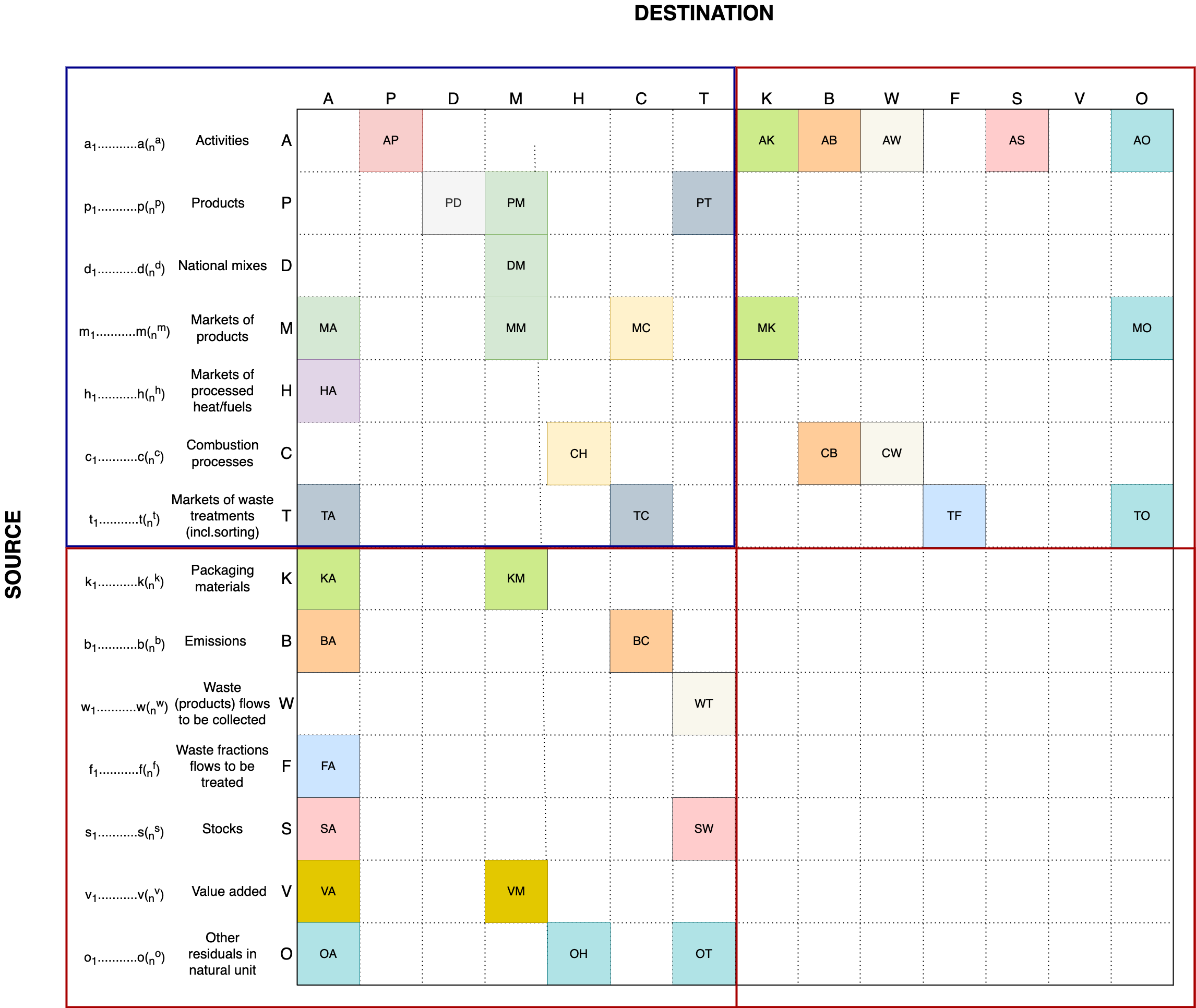
1. The Make-Use Framework

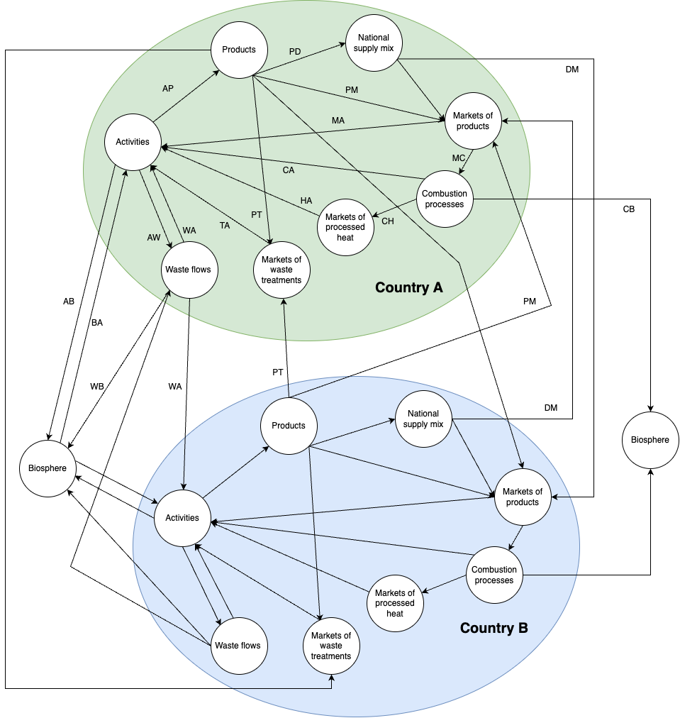
The following picture shows the structure of BONSAI-IO following the make-use framework (see the terminology in Glossary section):

An alternative illustration:

BONSAI aims to combine bottom-up and top-down data. The ultimate objective is to create an economy-wide analytical tool with strong technological consistency.

Bottom-up data are mainly production recipes, which we define as parameterized production functions (PPFs), retrieved from scientific literature, expert knowledge, and similar sources. The goal is to create a robust structure of productive processes. Other data consist of product properties, such as calorific values and prices.

Top-down data are collected from official statistics, sectoral associations, trade registries, and other sources. The goal is to scale up production processes and include consumption vectors. Of course, top-down data are necessary to capture the dimensions of regional systems and to validate our results against official statistics.

With the balancing procedure we reconcile bottom-up and top-down data.

Parameterized Production Function

Parameterized production functions are the fundamental building blocks for make-use tables. They define the relationship between input factors and output factors for a production process. PPFs are embedded into the general make-use framework following the procedures described here

In practical terms, a PPF specifies the reference product of an activity, the required inputs per unit of output, possible co-products, and, where relevant, the associated emissions or other residual flows. The “parameterized” aspect means that the same production logic can be reused across locations or technologies while key parameters, such as yield, efficiency, moisture content, nutrient content, or emission factors, are updated from the best available data. This allows BONSAI to preserve a transparent process recipe while still adapting it to regional conditions and sector-specific evidence.

Readers who want more detail on the underlying production-function approach can consult the BONSAI PPF resources here and here.

For the moment we have only used linear production functions, which can be defined as production recipes. Nothing excludes the possibility of including other non-linear functions in the future.

Sectoral Modelling

Sectoral models can be considered as a set of PPFs that are applied to a broad group of activities that share similar characteristics.

Agriculture

BONSAI consolidates crop and livestock accounts from FAOSTAT and complementary national statistics. The agricultural workflows harmonise physical yields, land occupation, and by-products before embedding them in the make-use system. Allocation between co-products follows agronomic balances consistent with the parameterised production functions.

The use of fertilisers by agricultural activities is determined combining, use of ferilisers and harvested area with the use of fertilisers by main crop categories.

Emissions from fertilisers application are obtained using the IPCC 2019 Refinement to the 2006 IPCC Guidelines for National Greenhouse Gas Inventories (IPCC 2019, Vol.4, Chapter 11).

With regard to livestock, the IPCC gudelines (IPCC 2019, Vol.4, Chapter 10) are used for calculating the dry-matter intake and the consequent emissions.

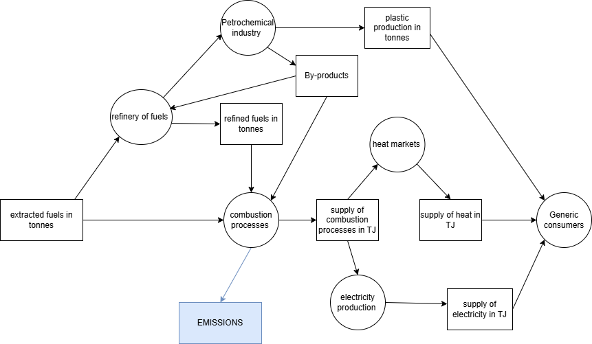
Energy

The energy module captures extraction, transformation, and delivery of fuels, heat, and electricity. Energy balances are reconciled with BONSAI activities by matching calorific values, technology efficiencies, and associated emissions, ensuring that physical and monetary layers remain coherent.

To improve transparency and traceability of emissions, ‘Combustion Activities (CAs)’ have been introduced. A combustion activity has (mass) fuels from the markets as inputs, and the generated heat as its reference flow. A combustion activity also produces emissions ans result of the combustion. Low heat values (lhv) are used for converting the mass of fuels into heat. Emission coefficients anf lhv are retrieved from EXIOBASE

Combustion activities exist for all fuels combusted in BONSAI locations. As a consequence of this approach, emissions are not directly attributed to fuel-consuming activities. To determine the direct emissions from fuel combustion in a specific activity, the combustion activity’s emissions must be multiplied by the demand of combustion activities in the activity. By doing so, it is possible to know exactly what is the source of the emissions. This approach diverges from convertional Input-Output databases, where emissions of an activities are grouped together and, if more fuels are combusted, it is not trivial to determine the source of them.

Below a diagram illustrates the modelling from fuel extraction till the final production of emissions:

Transport

The Transportation module is subdivided into two kinds of transport services: freight transport and passenger transport.

More about the methodology on the construction of the transport account here

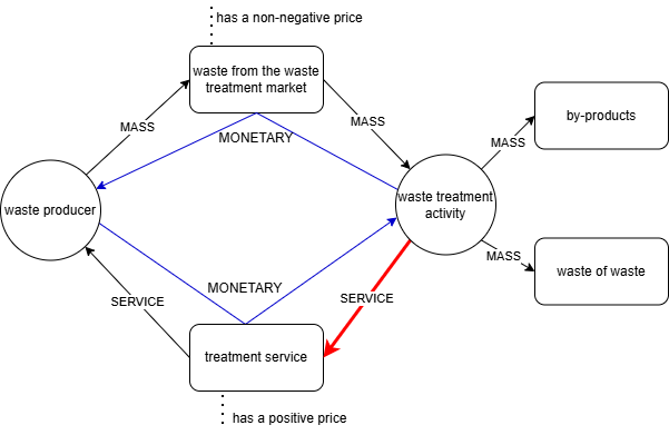
Waste treatment activities

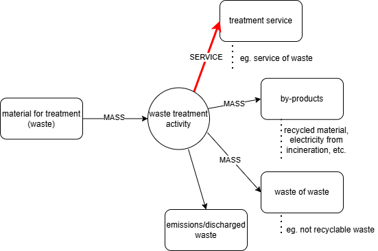
A waste treatment activity (WTA) is an activity that uses materials for treatment and delivers in return a waste treatment service. WTAs include:

• waste sorting

• recycling

• landfilling

• incineration

• wastewater treatment

• biogasification

• manure treatment

The reference flow (or the principal output) of a WTS is always assumed to be the service of treating waste. The treatment service is stricly linked to the incoming waste amount, eg. recycling of 1 kg of plastic waste. Other outputs linked to the input of waste can be:

• by-products: products that can be directly used as materials

• waste of waste: material for treatemnt that is sent to a another WTA

• emissions/discharged materials: mass that leaves the technosphere.

.

All the inputs and outputs to and from a WTA are always positive. This approach is consistent with both cases where a company pays to get rid of waste or, alternatively, gets some revenue from selling scraps. In BONSAI, it is assumed that two transactions occur between the waste producers and the waste treatment activity, which have different directions.

The first transaction is the “sale” of the material for treatment, while the second is the “sale” of the waste treatment service. In practice, it is assumed that both waste and service might have a positive price. The difference between these two transactions defines who pays whom.

.

The underlying idea is that the higher the quality of waste is, the higher the price a waste producer might get from selling the waste. If the quality is high, the waste producer can even gain from the sale of waste. The economic viability of the WTA will then come from the sale of the by-products.

Packaging

Basded on European Parliament and Council Directive 94/62/EC, packaging “means all products made of any materials of any nature to be used for the containment, protection, handling, delivery and presentation of goods, from raw materials to processed goods, from the producer to the user or the consumer”.

In BONSAI, we assume that each packaging has its own capacity, which can be considered as a service. For example a 50cl bottle provides the service of protecting 50cl of a liquid material.

Activities determine the required packaging based on their capacity needs. The volume of packaging is then converted into mass units. Consequently, activities receive a mass flow from packaging producers that equals the mass of the packaging required. In return, activities pay a corresponding monetary flow to the producers.

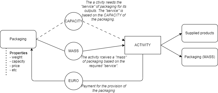
In BONSAI IO packaging supplied by activities to contain their output is reported in the extensions under specific packaging accounts. These packaging accounts describe the use and supply of packaging between suppliers and users. When packaging no longer provides its service, it becomes waste and is subsequently reported in the waste accounts as a regular waste flow.

Coefficients from Mass Flow Analyses

Related tasks:

distribute_using_general_distrib_coeff

Mass Flow Analyses (MFA) studies are used to distribute some specific products from which no information from PPFs or sectoral models is available. The MFA-derived distribution coefficients are used to allocate products to sectors. A mapping between MFA-activities and BONSAI-activities is performed to reconcile methodological differences and enable the use of MFA information. For exqmple, let us consider the steel used in buildings. In MFA, it might be assigned to different activities - such as companies or households - based on the typology of the building. In BONSAI, it would be allocated to construction sector, and only indirectly to activities through the use of construction services.

Coefficients from monetary tables

In BONSAI, there are several technical coefficients provided by PPFs, sectoral models and MFA. These coefficients are defined as exogeneous technical coefficients (EX-TC). However, the information coming from EX-TC mainly refers to the main inputs and outputs of activities. Therefore, to complete the recipes of activities, a complementary approach is used, based on Monetary Supply and Use tables. These coefficients derived with this approach are defined as endogeneous technical coefficients (EN-TC), which complement EX-TC.

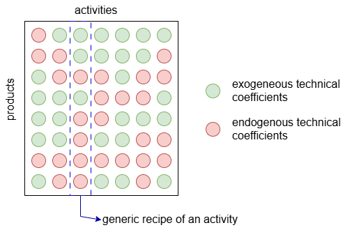
The procedure consists of distributing the residual product - not yet distributed via EX-TC - to the activities following the monetary technical coefficients.

residual product = total availability of a product - product distributed with EX-TC

where:

total availability = domestic supply + imports - exports.

The first step is, therefore, to calculate the residual product to distribute. Then, the monetary activities that have not yet assigned that product are selected, and distribution coefficients are determined based on the monetary use table. A distribution coefficient indicates how much of the residual product should be allocated to a specific monetary activity.

Because the the activity resolution of monetary tables is lower, each distribution coefficient is further divided accros BONSAI activities using principal (or determining) productions as weight. For example, if a distribution coefficient refers to the monetary sector electricity, it is further distributed to all the electricity producers in BONSAI.

Often, the product resolution in monetary tables is lower than that of BONSAI. Therefore, the same distribution coefficients can apply to several products. For example, if a distribution coefficient refers to the monetary product agriculture, it is used for all the agricultural products in BONSAI.

Trade and markets

The trade account is necessary to consider the bilateral exchanges between countries. We used COMTRADE, BACI and FAOSTAT as data sources.

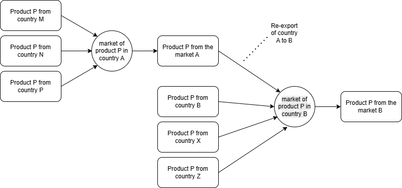
Differently from conventional multi-regional Supply and Use tables, BONSAI reports the trade with the introduction of markets.

Re-exports are re-allocated allowing a country to export the output of its own market. This ensures that flows contribute to either domestic markets or transit trade in line with the average market calculations described below.

Average Market

The average market account is calculated using production volume and trade data to estimate domestic market supply for each product. The formula is:

\[ V_{ij, \space \text{market supply}} = V_{ij, \space \text{domestic production}} + V_{ij, \space \text{import}} - V_{ij, \space \text{export}} \quad \text{for location } i \text{ and product } j \]

where,

• \(V_{\text{market supply}}\): is the total volume of domestic market supply.

• \(V_{\text{domestic production}}\): is the total domestic production.

• \(V_{\text{import}}\): is the total import.

• \(V_{\text{export}}\): is the total export.

It indicates that each product has its own domestic market, where domestic production and import are not differentiated. Additionally, re-exports need to be identified and adjusted as those goods do not contribute to the domestic market. Re-exports are identified using the following logic:

\[\begin{split} \text{HasReexport} = \begin{cases} 1, \quad \text{if} \quad V_{ij,\space \text{domestic}}+V_{ij, \space \text{import}} <= V_{ij,\space \text{export}} \\ 0, \quad \text{if} \quad V_{ij,\space \text{domestic}}+V_{ij, \space\text{import}} > V_{ij, \space\text{export}} \\ \end{cases} \end{split}\]

For locations that import a product from a re-exporting location, its import will be sourcing from the market supply of the re-exporting location instead of the industrial supply.

Electricity markets

Special treatment is given to the delineation of electricity markets. Electricity market is composed of two market: domestic production (i.e. the national mix) and import markets. The domestic production mix is composed of different domestic electricity generation technologies, e.g., solar PV, wind, and nuclear power. No individual markets are defined for each technology; all are grouped under the domestic production mix, i.e. the national electricity grid. The import market consists of electricity imported from foreign sources.

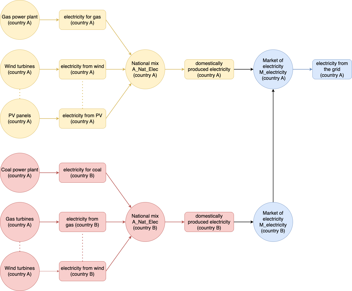
Besides national electricity markets, there are also regional energy markets. Currently, there are five regional markets, one for each continent. The role of regional markets is similar to that of global markets; what changes is the geographical resolution.

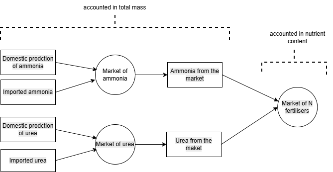
Fertiliser markets

There are three different markets providing nitrogen (N), phosphorus (P2O5) and potassium (K2O), respectively.

A fertiliser market is a special market because it is modelled as a market of markets. It receives fertilisers from the several markets of fertilisers and provides the nutrient to the users. Because the reference flow of the fertiliser market is accounted in nutrient content while fertilisers are accounted in total mass, a conversions occur. Nutrient-contents of fertilisers are used for that conversion.

Heat and fuel markets

Heat and fuel markets convert the heat from combusting several fuels into an unique value. Therefore, heat and fuel markets have several combustion activities as inputs, and heat as output.

Waste markets

Waste markets are defined for each waste fraction. Waste markets have the function of linking the waste producers, for example activities and households, to markets of waste treatment. The latter is just a normal market applied to waste treatment service produced by homogenous waste treatment activities. The method is stricly linked to waste input-output model.

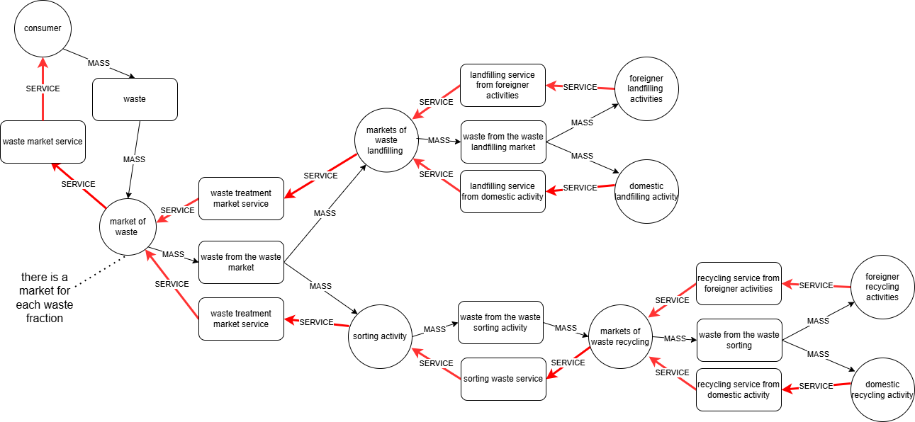
In the diagram, the presence of sorting activities can be noticed. The role of these activities is to include the footprint of the sorting process that would otherwise be excluded from the waste recycling service. Indeed, the real recycling of materials occurs in the virgin material sector. For example, the recycling of paper occurs when pulp from secondary paper is generated. In official statistics, the process of creating pulp from secondary paper is classified under the pulp production sector. However, the cost of waste sorting, according to offical statistics, is included in the waste sector, which is a separate sector. The latter also includes the final discharge of waste, such as incineration and landfilling. In BONSAI, when the inputs of the total monetary waste sector are distributed across the various waste treatment activities, the share of inputs associated to recycling processes will be allocated to the sorting activities.

Re-export

In modern economies, re-exports are common. An example is the re-export of avocados from the Netherlands to other European countries. BONSAI does not include a cleaning procedure to remove re-exports but instead aims to model them transparently.

A re-export occurs when a country exports a product without producing it. However, in BONSAI we also consider it a re-export when domestic production is too small to support both domestic demand and registered exports.

Re-exports are modeled by allowing countries to export their markets. This approach preserves the route of products from producers to consumers and provides a solid foundation for logistics modeling.

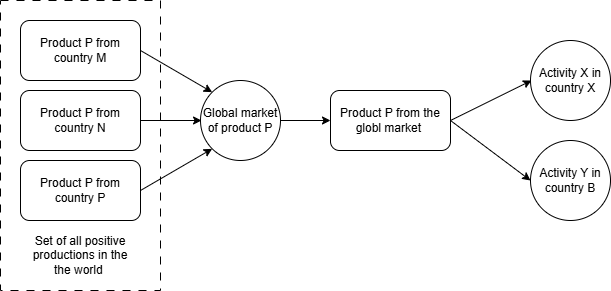
Global markets

When dealing with data from different sources, the chance of having conflicts of data is very high. One type of loop is when a set of countries do not carry out a product but from trade statistics we get that they only trade between them.

To solve this type of loops, global market are introduced. The underlying idea is that the markets causing the loop are replaced by global markets. A global market is made of all positive productions from the world regions.

Waste Accounts

Waste accounts define the use of supply of material for treatment by activities, final consumers. Waste accounts are inserted in the extensions of the Supply and Use tables. In other words, the waste accounts include all the mass flow that is exchanged between producers of waste, waste markets and waste treatment activities.

Waste accounts include:

• Waste supply: quantity of materials for treatment leaving producing activities, reported by product and origin.

• Waste use: quantity of materials for treatment entering treatment activities, capturing both physical flows and associated revenues.

In BONSAI, the supply of waste is an endogenous value obtained by applying different approaches, which are described below. Contrarily, the use of waste is mainly collected from official statistics. In many cases, the use of waste is larger than the supply of waste. For those cases, it is assumed that waste can come from stocks. A typical example is construction waste.

The supply of waste is determined using a lifetime function of products, which defines the time span when the total input of a product will be completely discharged as waste. Below an example of a lifetime function:

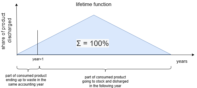
The lifetime function enables the calculation of the share of the products that will be discharged or accumulated into the stocks and become waste in the following years.

Material for Treatment

In BONSAI we use a definition of waste that was initially introduced in the FORWAST project. Waste refers to material for treatment that is a by-product of activities that needs a further treatment before being able to replace other materials.

Materials for treatment include waste flows but also scraps that are sold by activities who gain some revenues. In some occasion, for simplicity, the term waste is still used in BONSAI but indicates a material for treatment. Material for treatment are never a reference flow of an activity .

Food waste

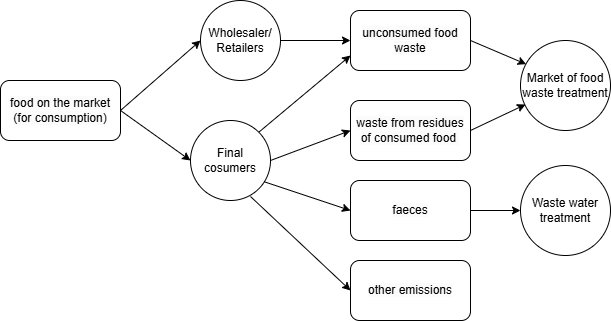
Food is a perishable product, and a portion of it ends up as waste without being consumed. Food waste occurs throughout the entire distribution chain, from wholesalers to final consumers.

In BONSAI,it is assumed that trade intermediaries have a food input equal to the amount they directly discharge as waste. This waste amount is then deducted from the food available to final consumers. The amount of food waste produced during the distribution chain is taken from USDA. Below a diagram of the approach used:

.

Waste from embodied products

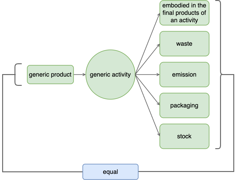
Flows used by activities are divided into two groups, embodied and not embodied. An embodied product is a product that can partially, or completely, end up in the principal product or in the by-product of an activity. Waste from embodied products is, therefore, the residual part of the flow not embedded. By doing so, it is implicitly assumed that residual part of embodied products is not accumulated in the stocks.

The waste of waste, which is the waste created by waste treatment activities when dealing with waste flows, is a subset of this group.

Waste from not-embodied products

Related tasks

determine_waste_coeff_of_residual_input,split_waste_and_stock_addition

Products that are neither embodied nor combusted are treated as potential waste. Then, using the lifetime functions, the latter is divided into discharged waste and stock addition, which will become waste in the following years. Therefore, a stock formation account of intermediate uses is created.

This approach diverges from the common practice in the input-output literature, where the formation of stocks is only included in the final consumption vector. In the conventional input-output tables, the intermediate uses are assumed to all have a lifetime of one year. This rule, which is mostly driven by accountability principles, refers uniquely to the economic lifetime of goods and may diverge from the physical lifetime considered in BONSAI.

The waste of packaging, which is the waste created when the packaging is discharged by the consumers, is a subset of this group.

Waste from combusted products

The residual solid part of a product that is left after the combustion, is defined as ‘ash’. The amount of this residual part is calculated using the ash content of products.

Emissions

The emission account compiles data on the direct emissions produced by various activities. This account is constructed by combining information from the product supply account and the emission coefficient account. Specifically, it quantifies emissions based on the total supply of principal products and the corresponding emission coefficients for each activity.

The emissions are calculated using the following formula:

\[ B = E \cdot \operatorname{diag}(V_{d}) \]

• \(B\): is the emission matrix that represents direct emissions of activities.

• \(E\): is the emission coefficient matrix that represent direct emission coefficient of activities.

• \(V_{d}\): is the vector of diagonal entries of the supply matrix.

The emission coefficient account is compiled from datasets including bonsai-ipcc, national emissions inventories, and sector-specific studies.

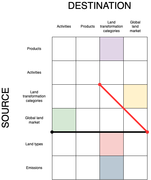
Land Use

There are

• Grass land

• Arable land

• Forest land
  The currently used data source for land use (FAOSTAT) includes the following types of forestry land: primary forest, secondary forest, planted forest, and naturally regenerated forest. In the land use module, we re-classify those forest lands into three categories:

  • Unmanaged forest

  • Extensively managed forest

  • Intensively managed forest

  First, the theoretical maximum area of managed forest is calculated as:

  \[ Area_{\text{manage, max}}=\frac{WR}{Y_{\text{min}}} \]

  where:

  • \(WR\): is the annual wood removal (\(m^3\)) in a country.

  • \(Y_{\text{min}}\): is the minimum yield of managed forests in a country (\(m^3/ha*year\)). This is defined as 1 \(m^3/ha*year\) weighted with potential productivity (based on \(NPP0\)).

  1. If \(Area_{\text{manage, max}}\le(Area_{\text{plant}})\)

     • the area of intensively managed forest \(Area_{\text{int}}=0\),

     • the area of extensively managed forest \(Area_{\text{ext}}=Area_{\text{manage, max}}\), and

     • the area of unmanaged forest \(Area_{\text{unmanaged}}=Area_{\text{prim}}+Area_{\text{sec}}+Area_{\text{nat}}\)

  2. If \(Area_{\text{plant}}<Area_{\text{manage, max}}\le(Area_{\text{plant}}+Area_{\text{nat}})\)

     • the area of intensively managed forest \(Area_{\text{int}}=0\),

     • the area of extensively managed forest \(Area_{\text{ext}}=Area_{\text{manage, max}}\), and

     • the area of unmanaged forest \(Area_{\text{unmanaged}}=Area_{\text{prim}}+Area_{\text{sec}}+(Area_{\text{plant}}+Area_{\text{nat}}-Area_{\text{manage,max}})\)

  3. If \(Area_{\text{manage, max}}>(Area_{\text{plant}}+Area_{\text{nat}})\)

     • Then, the area of intensively managed forest \(Area_{\text{int}}\) is calculated as follows:

       \[ Area_{\text{int, max}} = \frac{WR - (Area_{\text{nat}} + Area_{\text{plant}}) \cdot Y_{\text{min}}}{Y_{\text{int}}} \]

       where:

       • \(Area_{\text{int,max}}\): is theoretical max area intensive managed forest (ha*year) in a country.

       • \(Y_{\text{int}}\): estimated standard yield of intensive managed forests in a country (\(m^3/ha*year\)). This is defined as 4 \(m^3/ha*year\) weighted with potential productivity (based on NPP0).

       \(Area_{\text{int}}=min[Area_{\text{int,max}}, (Area_{\text{nat}} + Area_{\text{plant}})]\)

     • The area of extensively managed forest \(Area_{\text{ext}}=(Area_{\text{nat}} + Area_{\text{plant}})-Area_{\text{int}}\)

     • The area of unmanaged forest \(Area_{\text{unmanaged}}=Area_{\text{prim}}+Area_{\text{sec}}\)

Other natural resources

The accounting of the flows from the environment to the technosphere is also included in BONSAI-IO. Fossil fuels, mining products, nutrients from the ground, carbon absorbed by plants, and other natural resources are all part of natural resources accounts.

Value added

The use of primary factors, such as labour and capital, by each activity are also included.

Properties of products

The property account includes the conversion factors to convert a product flow across different property layers. It includes the following conversion factors:

• Price

• Heat value

• Weight

• Dry matter content

Balance

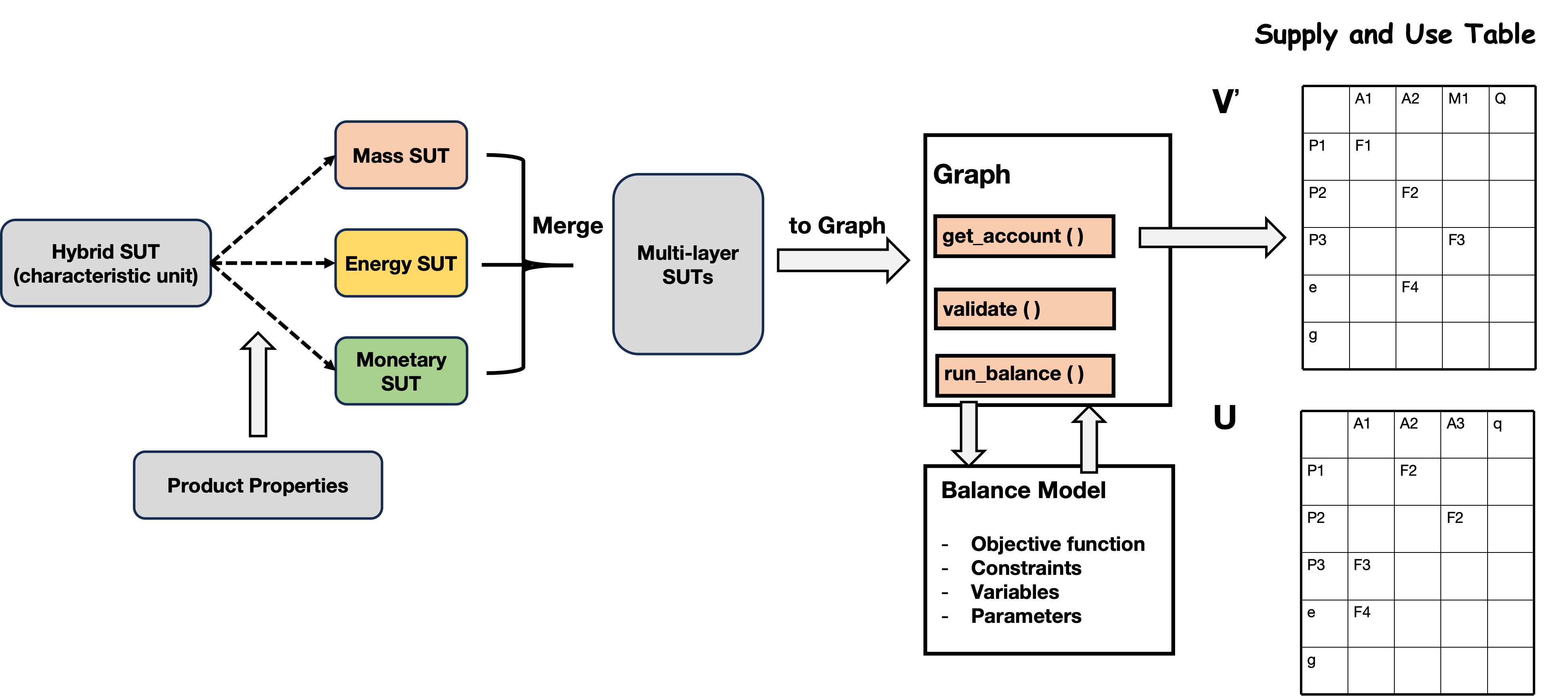
A graph-based multi-layer SUT balance framework is developed to balance the hybrid supply and use tables, as shown in the figure below:

The balance problem is formulated as follows:

\[\begin{equation*} \begin{aligned} \min_{\alpha, \beta} \quad & \sum_{i=1}^{I} \sum_{j=1}^{J} \sum_{k=1}^{K} |v_{ijk}| (\alpha_{ijk} - 1)^2 + \sum_{i=1}^{I} \sum_{j=1}^{J} \sum_{k=1}^{K} |u_{ijk}| (\beta_{ijk} - 1)^2 \\[6pt] \text{subject to:} \quad & \sum_{j=1}^{J} v_{ijk} \alpha_{ijk} = \sum_{j=1}^{J} u_{ijk} \beta_{ijk}, && \forall i,\ \forall k, \\[4pt] & \sum_{i=1}^{I} v_{ijk} \alpha_{ijk} \leq 10 \sum_{i=1}^{I} u_{ijk} \beta_{ijk}, && \forall j,\ \forall k, \\[4pt] & v_{pj k^{*}} \alpha_{pj k^{*}} = r_{b, j}\, v_{bj k^{*}} \alpha_{bj k^{*}}, && \forall j, \\ & && \forall p, b \in P_j,\ p \neq b,\ \text{s.t. } r_{b, j} \text{ is defined}, \\[4pt] & v_{pj k^{*}} \alpha_{pj k^{*}} = a_{q, j}\, u_{qj k^{*}}\, \beta_{qj k^{*}}, && \forall j, \\ & && \forall p \in P_j,\ \forall q \in P_j,\ p \neq q,\ \text{s.t. } a_{q, j} \text{ is defined}, \\[4pt] & \underline{v}_{pjk^{*}} \le v_{pjk^{*}}\alpha_{pjk^{*}} \le \overline{v}_{pjk^{*}}, && \forall j = 1,\dots,J,\ \forall p \in P_j, \\[4pt] \end{aligned} \end{equation*}\]

where:

• \(\alpha_{ijk}\): Adjustment factor for supply of product \(i\), activity \(j\), and unit \(k\).

• \(\beta_{ijk}\): Adjustment factor for use of product \(i\), activity \(j\), and unit \(k\).

• \(v_{ijk}\): Initial supply volume of product \(i\) by activity \(j\) in unit \(k\).

• \(v_{ibk}\): Initial supply volume of the base/determining product \(b\) by activity \(j\) in unit \(k\).

• \(u_{ijk}\): Initial use volume of product \(i\) by activity \(j\) in unit \(k\).

• \(P_j\): Set of products co-produced by activity \(j\).

• \(r_{b, j}\): By-product ratio indicating by-product \(b\) produced per unit of reference product &p& by activity \(j\) (\(v_{bjk}/v_{pjk}\)).

• \(a_{q, j}\): Technical coefficient between reference product

• \(k^{*}\): The characteristic unit/layer of supply/use.

Constraints

• Product Balance ensures total supply of a product equals its total use.

• Activity Balance ensures total input to an activity does not exceed its total output.

• Output Ratio Constraint ensures the ratio of co-produced products for an activity remains constant.

Flow balance

Flow balance enforces that, for every product and property layer, the balanced supply equals the balanced use of each node in the graph. The optimisation scales upstream and downstream flows along the network until conservation holds within acceptable tolerances, using the structure illustrated above.

Activity balance

It is imposed that for each input to an activity the following condition holds:

After balance disaggregation

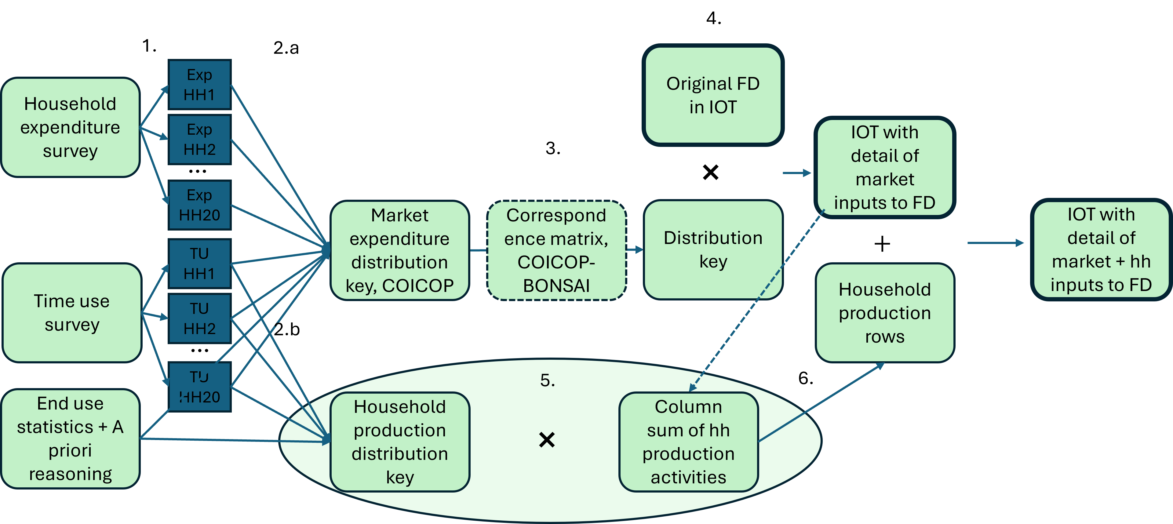
Household

The household production and consumption are disaggregated via distribution keys generated by household expenditure and time-use survey following the formula below.

For the use matrix:

\[ U_{f} = D_{use}^{T}f \]

where:

• \(U_{f}\): is disaggregated use matrix by household, with dimensions \(p \times a\).

• \(D_{use}\): is the market use distribution key matrix of size \(p \times a\), containing non-negative elements no greater than 1. A market use distribution key \(d_{p,a}\) shows the percentage of each product used per household group-activity with each summing to 1

\[ \sum_{a}(D_{supply})_{p,a}=1,\quad \forall p \]

• \(f\): is the household final demand vector of dimensions \(p \times 1\).

For the supply matrix:

\[ V_{w} = D_{supply}w \]

where:

• \(V_{w}\): is disaggregated household supply matrix, with dimensions \(a \times p\).

• \(D_{supply}\): is the product supply distribution key matrix of size \(p \times a\), containing non-negative elements no greater than 1. A market use distribution key \(d_{p,a}\) shows the percentage of each product used per household group-activity with each summing to 1

\[ \sum_{a}(D_{supply})_{p,a}=1,\quad \forall p \]

• \(f\): is the labor supply vector of dimensions \(p \times 1\).

The full workflow to disaggregate the household production and consumption is as follows:

2. Transformation into Input-Output tables

The compiled make-use system is only a mirror of the past biosphere-technosphere interactions, to serve the accounting purpose. Therefore, it only serves as a descriptive tool.

If the aim is to estimate the footprints of products or processes, some assumptions must be adopted. Therefore, we move from an accounting tool to a modeling one.

In practice, this process consists of linking users and producers of products. This apparently simple transformation is purely subjective and there is a long literature on how to proceed.

There are three main approaches to transform make-use into input-output tables:

• By-product technology model (Stone’s method)

• Product technology assumption

• Industry technology assumption

Here we have decided to implement the by-product technology model. This approach, developed within the Input-output community, has been adopted by the consequential LCA practitioners because it better models the causal-effect link associated with behavioural changes. Within LCA community, the Stone’s method is defined as system expansions.

By-product Technology Modelling

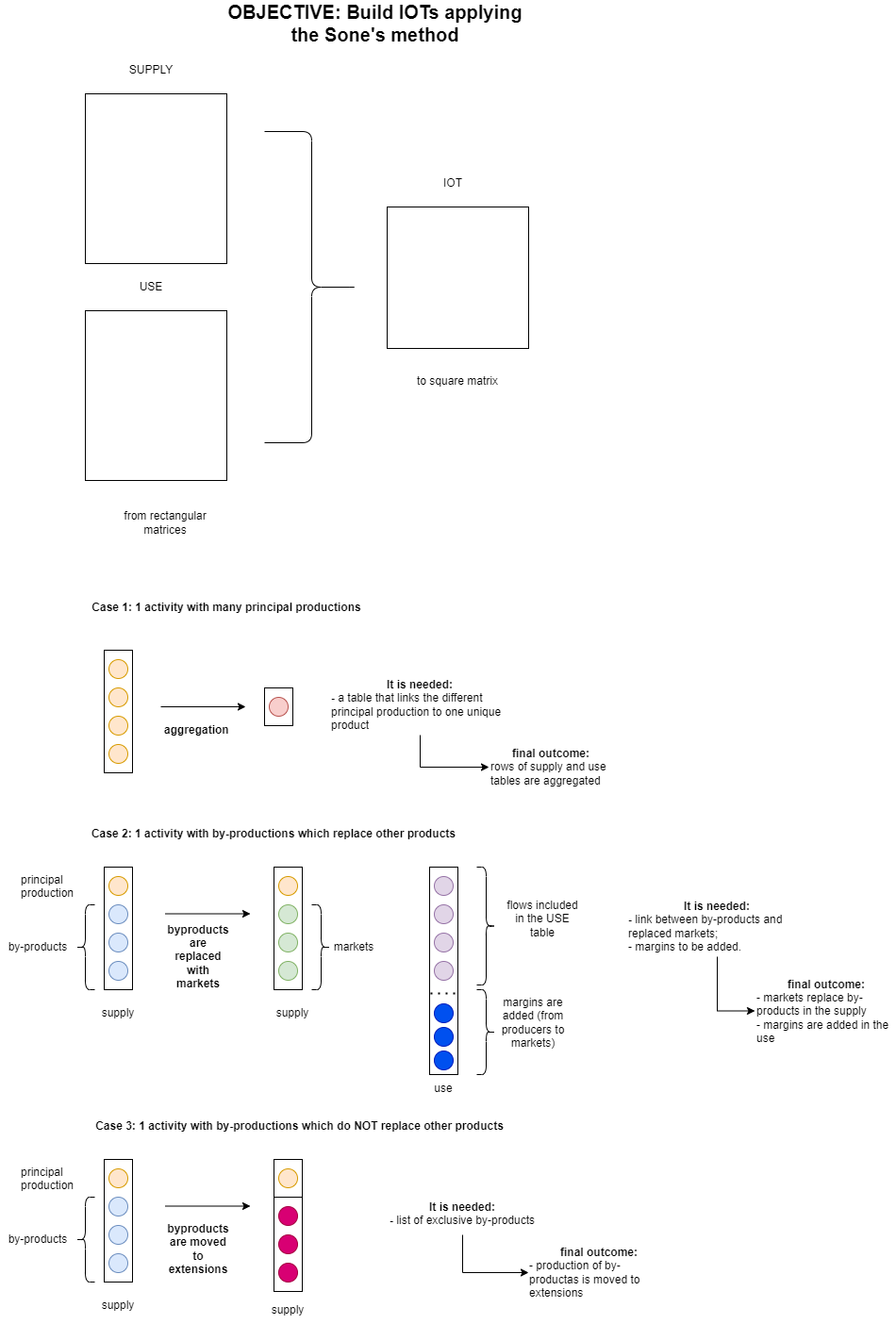
The formula is given as:

\[ m = B\cdot(V_{d}^{T}-(U-V_{od}^{T}))^{-1}\cdot k = B\cdot(V^{T}-U)^{-1}\cdot k \]

where:

• \(m\): is the environmental intervention, meaning the total of direct and indirect environmental impact, of a product of interest.

• \(B\): is the direct emissions of activities.

• \(V_{d}\): is the vector of diagonal entries of the supply matrix.

• \(V_{od}\): is the off-diagonal entries of the supply matrix.

• \(U\): is the use matrix.

• \(k\): is a vector of products, in which all entries are zero, except the entry for the product of interest.

3. Consequential modelling

The compiled make-use system is only a mirror of the past biosphere-technosphere interactions, to serve the accounting purpose. Consequential modelling aims to model the causal-effect link associated with behavioural changes, i.e., how a marginal change in demand affects upstream supply. The system is then transformed and extended for causal-effect linking, following the consequential modelling requirements in the ISO 14040 and 14044.

The steps to move from the accounting system to the consequential system includes the following steps:

• By-product technology model as defined above

• Marginal producers

• Indirect land use change model

• Marginal electricity model

• Capital endogenization model

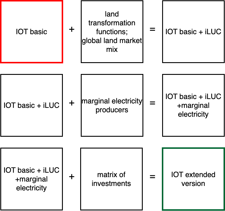
Indirect land use change

Marginal Electricity Mix

Implementation details for the marginal electricity workflow are documented alongside the workflow tasks referenced above. The direct requirement matrix \(A\) for the marginal electricity mix is given by:

\[ A = (V^{T}-V_{\text{elec, base}}^{T}+\Delta{V_{\text{elec}}^{T}}-U)\cdot(V^{-1})^{T} \]

where:

• \(A\): is the direct requirement matrix.

• \(V\): is the supply table.

• \(V_{elec, base}\): is the base electricity supply matrix, representing the initial state of electricity supply.

• \(\Delta{V_{elec}}\): is the marginal electricity supply matrix.

• \(U\): is the use matrix.

The marginal electricity supply is calculated following the logic as follows:

\[ \Delta{V_{elec}} = V_{\text{elec, base}} \circ M_{\text{elec}} \]

• \(V_{\text{elec, base}}\): Base electricity supply matrix, as defined above.

• \(M_{\text{elec}}\): Marginal electricity supply matrix, representing the marginal increase in supply of different electricity supply activities responding to the unit increase in electricity demand.

• \(\circ\): Denotes element-wise (Hadamard) multiplication.

The marginal electricity supply matrix is then calculated as:

\[\begin{split} M_{\text{elec}} = \begin{cases} \frac{v_{j, \text{future}} - v_{j, \text{base}}}{v_{j, \text{base}}(t_{future}-t_{base})} & \text{if} \quad \frac{v_{j, \text{future}} - v_{j, \text{base}}}{v_{j, \text{base}}(t_{future}-t_{base})} \ge \delta\\ 0 & \text{if} \quad \frac{v_{j, \text{future}} - v_{j, \text{base}}}{v_{j, \text{base}}(t_{future}-t_{base})} < \delta \\ \end{cases} \end{split}\]

where:

• \(v_{j, \text{base}}\): Base value of the electricity supply activity \(j\)

• \(v_{j, \text{future}}\): Future value of the electricity supply activity \(j\)

• \(t_{base}\): Initial time period.

• \(t_{future}\): Future time period.

• \(\delta\): The capital replacement rate/depreciation rate below which the marginal increase is considered negligible and thus set to zero.

The future electricity supply is extrapolated based on a net-zero for 2050 scenario from the Global Change Assessment Model (GCAM v6.0) in the NFGS version 4.0 scenario dataset. The scenario assumes that all pledged targets by countries globally to UNFCCC, even if not yet backed up by implemented effective policies. For detailed assumptions and methodology, refer to the documentation.

Capital Endogenization

Implementation notes for capital endogenization are provided in the capital-related workflow tasks referenced above. The flow matrix approach is applied to endogenize capital goods for footprint assessment, as summarised below. Specifically, the requirement of capital goods by current intermediate activities is added into the requirement matrix using the following formula:

\[ A = (V_{d}^{T}+V_{od}^{T}-U-U_{C})\cdot(V_{d}^{-1})^{T} \]

where

• \(A\): is the direct requirement matrix.

• \(V_{d}\): is diagonal entries of the supply matrix.

• \(V_{od}\): is off-diagonal entries of the supply matrix.

• \(U\): is the use matrix.

• \(U_{C}\): is the capital use matrix, which represents the use of capital goods by current intermediate activities.

The capital use matrix \(U_{C}\) captures the inputs of capital goods in the production of current intermediate activities. It can be calculated from gross fixed capital formation (GFCF) by different capital goods and total consumption of fixed capital (CFC) by current intermediate activities. First, the capital use matrix is derived from the matrix multiplication of the capital requirement matrix and the diagonization of GFCF vector:

\[ U_{K} = K \cdot \hat{GFCF} \]

where

• \(K\): is the capital requirement matrix where its element \(k_{ij}\) represents the share of a capital goods required by an industrial activity. The row sum of the capital requirement matrix shall be either one (has capital goods used by the activity) or zero (no capital goods used by the activity).

• \(\hat{GFCF}\): is the diagonalization of the GFCF vector.

The capital requirement matrix is calculated based on consumption of fixed capital as follows:

\[ K = \hat{(I \cdot \hat{d} \cdot e)}^{-1} \cdot I \cdot \hat{d} \]

where

• \(I\): is a virtual investment matrix recording the use of capital goods/investment by current intermediate activities.

• \(d\): is the vector of total consumption of fixed capital by current intermediate activities.

• \(e\): is the summation vector in proper dimensions.

4. Glossary

• Activity: Doing or making something.

• Product: Output of an activity with a positive market or non-market value (utility).

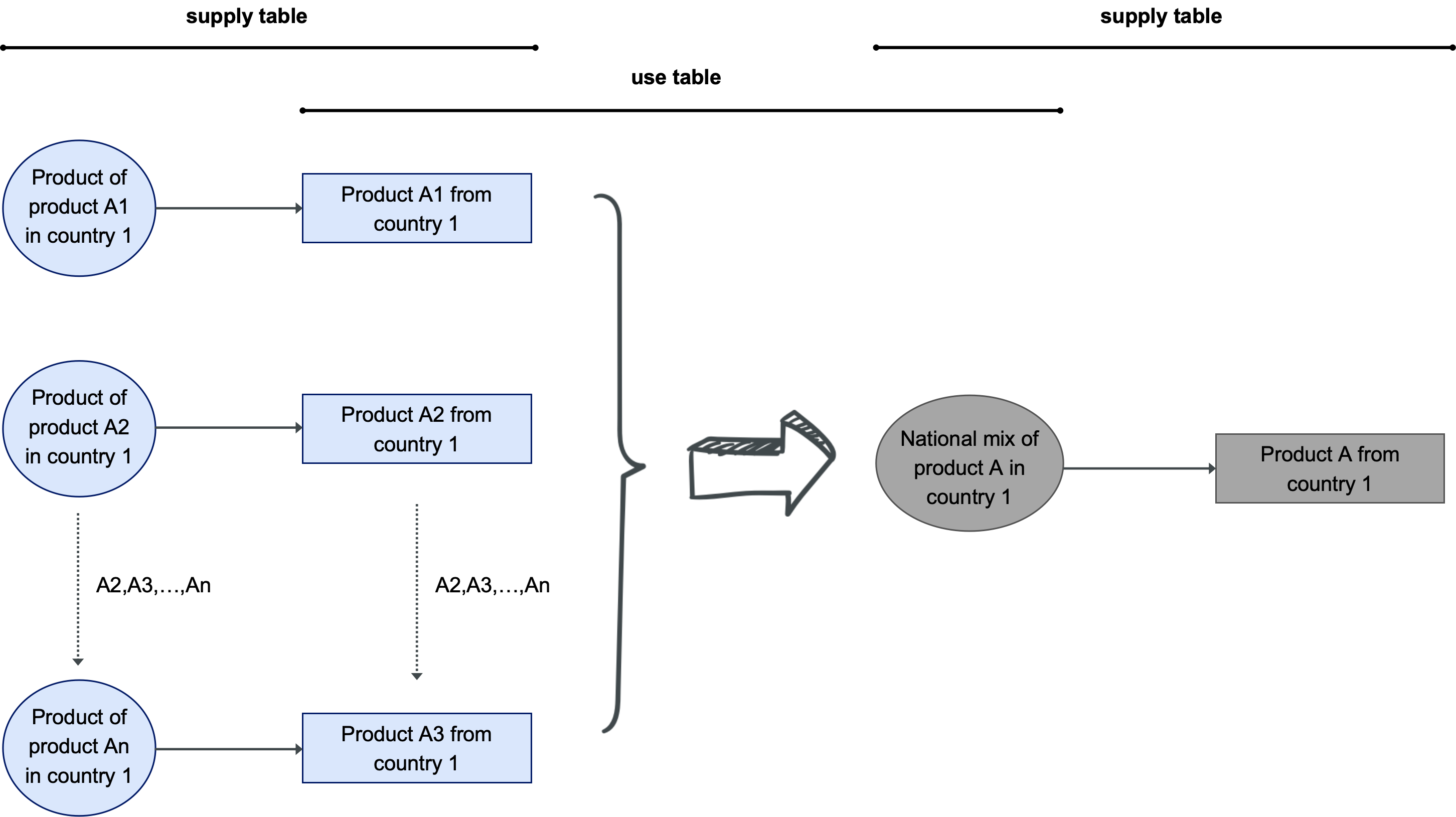
• National mixes: collects homogeneous products from several sources and produces one unique (mixed) product. The output of the national mix is always associated to the lowest product resolution which can be obtained combining trade accounts and use tables. If homogenous products from different producers are not exported from one region to another, there is no need of creating a national mix. Those products will feed to the national markets.

Note

A national mix differs from market because it does not include trade and sale margins, plus net taxes on products.

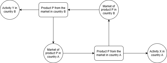
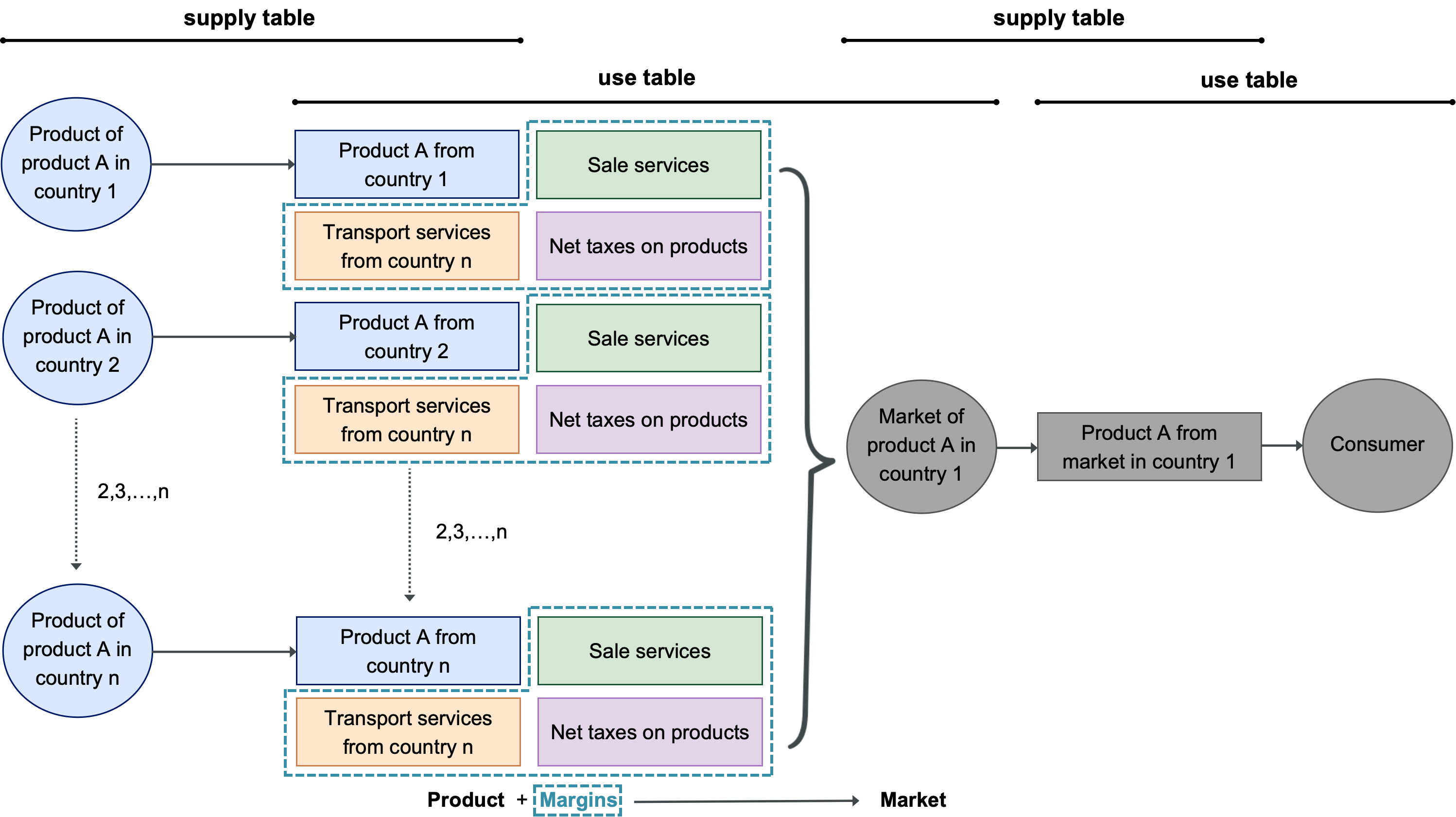
• Market activity

  A market activity is an intermediate activity between producers and users where basic prices are converted into purchaser prices. Producers from several countries (exporting activities) feed products to a national market (importing country). Other inputs to the markets are:

  • the transport services to move the products from the origin country to the destination one;

  • trade services which includes all the other margins of the trade intermediaries;

  • net taxes on products.

• Markets of products: These are aggregate representations of similar products from various producers (e.g., steel from multiple manufacturers), pooled into a market to reflect the typical product mix available for use. They account for average properties, emissions, or energy use across producers.

• Markets of processed heat/fuels: These are specific types of product markets focused on thermal energy or fuel types (e.g., district heat, diesel, biogas), reflecting aggregated supply from multiple production routes or regions. These markets smooth over differences in source inputs to provide an average supply characteristic.

• Combustion processes: These represent specific technological activities where fuels are burned to produce energy, heat, or mechanical work — and are a major source of emissions inventories (e.g., industrial boilers, residential stoves, or vehicle engines). Each combustion process typically has a distinct emissions profile depending on fuel type and technology.

• Markets of waste treatments: These are modeled entities representing how different waste streams (e.g., municipal solid waste, hazardous waste, sewage sludge) are typically treated — via incineration, landfilling, recycling, composting, etc. They can represent national average treatment pathways for specific waste types.

• Packaging materials: Materials used to protect or contain products (e.g., plastic film, cardboard, glass bottles). They are modeled as separate product flows because they have distinct life cycles and disposal routes and significantly influence waste generation and recycling rates.

• Emissions: These are residual flows from processes to the environment (the biosphere). Emissions include CO₂, NOₓ, particulate matter, heavy metals, etc., and are typically tracked in physical units (e.g., kg/year). They are crucial for assessing environmental impacts.

• Waste (products) flows to be collected: These are post-consumer flows of products that become waste and are collected by waste management systems. This includes recyclable materials, organic waste, or non-recyclables — typically in mixed or sorted streams.

• Waste fractions flows to be treated: After collection, waste is sorted into fractions (e.g., plastic, glass, organics) and sent to treatment processes (e.g., mechanical sorting, pyrolysis, composting). These flows represent the routing of specific waste types to their respective treatment technologies.

• Stocks: Physical quantities of materials or products that are accumulated in the economy but not immediately consumed or disposed. This includes construction materials in buildings, cars in use, electronics in households, etc. Stocks influence future waste generation and resource demand.

• Value added: This is the economic contribution of a production activity — typically measured as output minus intermediate consumption. It includes wages, profits, and taxes, and is crucial in linking physical flows with monetary input-output models.

• Other residuals in natural unit: These include non-emission, non-waste residual flows, such as heat losses, rejected water, noise, or byproducts in physical terms (e.g., MJ, liters, kg) that don’t fit into conventional product or emission categories but are still environmentally relevant.

Data sources

Account	Source	Accessed
> Production
Crops and livestock products	FAOSTAT	03/2023
Use and supply of Crops and livestock products	FAOSTAT	10/2024
Extraction of minerals	UN IRP (2021)	09/2021
Forestry	FAOSTAT	08/2021
Fishery	FishStat	12/2021
Manufactured products	UNSD	11/2021
Manufactured products (EU)	PRODCOM	12/2021
Manufactured products (CN)	CBS-China
Basic metals and ores extraction	USGS	06/2024
Basic metals and ores extraction	BGS	03/2021
Fertilizers by product	FAOSTAT	03/2023
Fertilizers by nutrients	FAOSTAT	03/2023
Motor vehicles	OICA	12/2021
Waste treatment services - municipal (Europe)	EUROSTAT	06/2024
Waste treatment services - municipal (US)	EPA
Secondary steel	Worldsteel

Quality assurance

Quality assurance in BONSAI combines internal consistency checks in the hybrid supply-use model with external validation and release-to-release review. The balancing framework is central, but they are complemented by benchmark comparisons, anomaly screening, and workflow-specific checks.

• The balance framework

  Because the starting data are assembled from different sources, production statistics, trade data, and activity recipes do not always align in the first assembled system. Therefore, we introduce the balance framework reconciles the hybrid supply-use system so that the final tables satisfy the core accounting relationships of the entities represented in the model. The system is modelled as a graph of activities and products connected by flows in multiple property layers. The balancing variables act on the supply and use flows themselves: each original flow is associated with an adjustment factor, initialized at 1, that can scale the flow upward or downward. The balancing problem then searches for the set of adjustments that restores consistency while keeping the balanced system as close as possible to the original data. The core balance constraints are:

  • Product balance: for each product in its characteristic physical layer, total balanced supply must equal total balanced use (a hard constraint). For example, if 1000 kg of wheat are available after production and imports, the balanced uses of wheat must also sum to 1000 kg.

  • Activity balance: each activity must remain feasible when its inputs and outputs are considered together. In practice, the model constrains the relationship between total inflows and total outflows so that markets do not supply more than they receive, and production activities remain within plausible input-output ranges. Unlike product balance, this is not a strict equality constraint but a bounded feasibility condition.

  • Cross-layer consistency: Flows exist both in a physical layer and in the monetary layer. Therefore, the model also limits how far the implied price can move from its initial value. Here, the implied price is the monetary flow divided by the corresponding physical flow, with the initial value coming from an internally maintained price dataset. This prevents the model from resolving a physical consistency by creating monetary inconsistency.

  Putting together, the model searches for the adjusted flows that satisfy the balancing identities while minimizing the weighted deviation from the original values. In practice, large discrepancies in raw data mean that not all accounting and technical constraints can always be enforced simultaneously across the full system. BONSAI therefore uses repeated balancing experiments to identify the largest set of constraints that the available data can satisfy while still producing the most coherent system possible. In the current implementation, this is handled selectively for the main balance controls as follows:

  • For product balance: the constraint is applied only in the product’s characteristic physical layer, currently the mass layer, and is skipped for cases with very large initial mismatches (20 times difference) between supply and use. This avoids forcing exact balance in parts of the system where the raw data are too contradictory for the balance to converge.

  • For activity balance: the constraint is enforced as a set of feasibility inequalities rather than a strict equality. The model constrains the relation between total inflows and total outflows so that activities remain plausible, but it allows different tolerances depending on the type of activity and layer. Specifically, market activities are kept close to one-to-one balance, while production activities are balanced under broader ranges especially within the monetary layer, reflecting the fact that monetary flows can be more uncertain than physical flows (considering price uncertainties). The constraint is also skipped for activities with missing reference products and missing inflows or outflows, does not could lead to inconvergence.

  • For cross-layer balance: cross-layer consistency is currently enforced only for a selected subset of links between physical flows and monetary flows, through price-feasibility constraints for specific product groups (around 20 products). This selective approach is necessary because adding price constraints causes the size of the optimization problem to grow very rapidly, beyond what can currently be handled on a single compute node. We need more capable computing infrastructure and seek ways to optimize the underlying model data structure to support larger balancing models in future releases.

• Technical constraints

  Alignment with accounting identities does not by itself guarantee that the resulting system is technologically or physically credible. BONSAI therefore introduces technical constraints as an additional guardrail within the balancing framework to keep the balanced system technologically and physically grounded.

  In practice, these constraints are defined around the reference product of each activity and express known relationships between that reference output and its required inputs or associated co-products. For example, if 1 kg of cheese is known to require at least 4 kg of milk, the balanced recipe should not violate that minimum input requirement. These relationships are maintained in an internal technical-constraint dataset containing nearly 90,000 records. The dataset is updated incrementally. New information is appended only, and where records overlap, the most recent entry supersedes earlier ones.

Additional quality assurance steps complement the balancing model:

• Cross-validation of production and trade data

  Before the final supply and use tables are generated, dedicated preprocessing tasks reconcile production statistics with bilateral trade data. This step is needed because the balancing framework adjusts flow magnitudes within the existing network, but does not create or reroute links between activities and products. The adjustment therefore resolves structural inconsistencies upstream, including explicit treatment of re-exports and scaling or redistribution procedures when reported trade would otherwise imply impossible or inconsistent market supply.

• Emissions inventories validation

  After balancing, and before footprint calculation, aggregated direct emissions are compared at country level with external benchmark datasets such as EDGAR. These comparisons are used to detect systematic deviations in total emissions, identify possible gaps or drifts in the underlying accounts, and validate the overall consistency of the balanced system.

• Outlier and anomaly screening

  After footprint calculation, statistical screening is used to identify unusual footprint values and structural outliers using distribution-based methods, such as median-based thresholds. Detected anomalies are not only flagged for review, but can also be incorporated into the technical-constraint dataset, creating a feedback loop that gradually refines coefficient bounds and recipe structures. This helps reduce recurring inconsistencies and improve model robustness over successive runs.

• Version-by-version footprint comparison

  Furthermore, we include also a version-to-version footprint comparison procedure to assess how footprints change between releases. These checks are used to review random samples and broader result shifts against the previous version, helping distinguish expected methodological improvements from unintended regressions.

• Sanity-check benchmark footprint dataset

  Before each release, calculated footprints are compared against an internally maintained benchmark dataset. This benchmark is used to flag product footprints that fall outside expected ranges and to identify results that require manual review before publication.

These checks do not remove the need for expert judgement, but they substantially reduce the risk that invalid source data, inconsistent scaling, or unintended modelling errors propagate into the footprint data.

Further Reading

• Consequential LCA glossary

• bonsai.io portal

• Workflow implementations under src/bonsai/io/ (see module docstrings for details)